HMSPC: A Hybrid Mechanistic-Stochastic Physical-Continuous Model for Battery Dynamics
Code available at HMSPC GitHub
Preprint version now available at Zenodo!
Abstract
Battery voltage dynamics are irregularly sampled, noise-corrupted, and strongly regime-dependent, properties that challenge standard sequential models. I propose HMSPC (Hybrid Mechanistic-Stochastic Physical-Continuous Model), a continuous-time latent variable model that addresses these challenges through two key components: a gated input-conditioned latent ODE that explicitly incorporates exogenous observations (current and temperature) into continuous-time state evolution, and a heteroscedastic observation model with uncertainty regularization that produces calibrated predictive variance. Built on the Latent ODE[1] framework, HMSPC replaces purely autonomous latent dynamics with a learned gating mechanism that adaptively controls how strongly operating conditions influence trajectory evolution at each integration step. Evaluated on the MIT-Stanford dataset[2] against Latent ODE and Vanilla Neural ODE[3] baselines across 5 seeds, HMSPC achieves a mean RMSE of 32.37 $\pm$ 1.34 mV compared to 58.33 $\pm$ 4.19 mV for Latent ODE, yielding a 45% reduction, alongside well-calibrated uncertainty estimates (ECE 0.078). Ablation studies confirm that input-conditioned drift and heteroscedastic noise each contribute meaningfully to both accuracy and calibration.
1 Introduction
Lithium-ion batteries are central to the energy transition, powering electric vehicles, grid storage, and consumer electronics. Accurate modeling of battery voltage dynamics is critical for state-of-health estimation, degradation prediction, and safe operation. Yet battery data presents a fundamental challenge for sequential models: observations are irregularly spaced in time, corrupted by sensor noise, and strongly influenced by external driving conditions such as charging current and temperature.
Standard recurrent neural networks assume discrete, regularly spaced observations and autonomous internal dynamics, making them poorly suited to this setting. Neural ODEs address the irregular sampling problem by parameterizing hidden state evolution as a continuous-time differential equation, but their dynamics remain largely input-independent during the generative phase, providing poor inductive bias for systems where the trajectory is explicitly driven by external inputs. Latent ODEs extend this framework with variational inference over continuous latent trajectories, but inherit the same limitation.
Battery voltage dynamics are fundamentally regime-dependent: the same cell exhibits qualitatively different behavior under fast charging versus slow discharge, and at different temperatures. A model that ignores current and temperature during latent state evolution must recover this structure from the latent state alone, placing an unnecessary burden on the encoder and limiting generalization.
While Latent ODEs are probabilistic through their latent-variable formulation, they typically assume a fixed observation noise model and therefore do not provide input-dependent predictive uncertainty estimates. In safety-critical applications such as battery management, knowing how confident the model is matters as much as the prediction itself; overconfident predictions of remaining capacity or voltage bounds can lead to unsafe operation.
I propose HMSPC (Hybrid Mechanistic-Stochastic Physical-Continuous Model), a continuous-time latent variable model that directly addresses this gap. HMSPC augments the latent ODE with a gated input-conditioning mechanism: at each integration step, the drift is modulated by a learned gate that controls how strongly the current operating conditions influence latent state evolution. This allows the model to selectively incorporate input information when it is most informative, rather than applying fixed conditioning throughout. I further equip the decoder with a heteroscedastic observation model, where predictive variance is itself conditioned on the latent state and inputs, in contrast to the original Latent ODE formulation, which assumes a fixed isotropic observation noise. This allows uncertainty estimates to adapt to the operating regime, naturally expressing higher uncertainty during aggressive charging or at end-of-life where voltage dynamics are less predictable.
I evaluate HMSPC on the MIT-Stanford dataset against Latent ODE and Vanilla Neural ODE baselines, and conduct a systematic ablation study over the key architectural components. HMSPC achieves a mean RMSE of 32.37 $\pm$ 1.34 mV compared to 58.33 $\pm$ 4.19 mV for Latent ODE, alongside well-calibrated uncertainty estimates (ECE 0.078).
My main contributions are:
- A gated input-conditioned latent ODE that adaptively incorporates exogenous driving signals into continuous-time latent dynamics.
- A heteroscedastic observation model with an uncertainty regularization objective that produces calibrated, input-conditioned predictive variance, replacing the fixed isotropic noise assumption of standard Latent ODEs.
- Empirical demonstration of consistent gains over Latent ODE and Neural ODE baselines in both reconstruction accuracy and uncertainty calibration on real battery cycling data.
2 Background
Modeling irregularly sampled time series remains a persistent challenge in sequential learning, particularly in domains where observations are sparse, noisy, and unevenly spaced in time. Standard recurrent neural networks (RNNs) assume discrete and regularly spaced observations, limiting their applicability in such settings.
Neural Ordinary Differential Equations (Neural ODEs) generalize continuous-time dynamics by parameterizing hidden state evolution as a differential equation $\frac{\mathrm{d}z}{\mathrm{d}t} = f_\theta (z, t)$, allowing latent states to evolve continuously between observations. While this formulation naturally handles irregular time gaps, it assumes autonomous dynamics that are not explicitly conditioned on observed inputs during evolution.
To address this limitation, the ODE-RNN framework introduces discrete updates via recurrent units while maintaining continuous-time evolution between observations. Building on this idea, Latent ODEs replace the recognition network with an ODE-RNN encoder, enabling variational inference over continuous latent trajectories. Latent ODEs provide a principled probabilistic framework for irregular time series, but still rely on largely input-independent latent dynamics during the generative phase.
In practical applications such as battery state-of-health estimation, system dynamics are strongly influenced by external driving variables such as current and temperature, suggesting the need for explicitly input-conditioned continuous-time models. This motivates models that incorporate structured input-conditioning within continuous-time latent dynamics.
3 Method
3.1 Problem Formulation
I consider an irregularly sampled multivariate time series \(\{x_{t_i}\}_{i=1}^{T}\) with strictly increasing timestamps $t_1 < t_2 < \cdots < t_T$. Each observation is defined as:
\[x_{t_i} = \begin{bmatrix} V_{t_i} \\ I_{t_i} \\ \text{Temp}_{t_i} \end{bmatrix} \in \mathbb{R}^3\]where \(V_{t_i}\), \(I_{t_i}\), and $\text{Temp}_{t_i}$ are the observed voltage, current, and temperature at timestamp $t_i$ respectively. I additionally define a per-timestamp observation mask \(m_{t_i} \in \{0,1\}\), which applies jointly to all three channels denoting whether a timestamp is either fully observed or fully missing. Inter-observation time gaps are defined as \(\Delta t_i = t_{i+1} - t_i\) for \(i = 1, \ldots, T-1\). I denote the full observed sequence as \(\{x_{t_i}\}_{i=1}^{T}\).
3.2 Variational ODE-RNN Encoder
The encoder maps the observed sequence to a distribution over the initial latent state $z_0$. It does so by maintaining a latent hidden state $h(t) \in \mathbb{R}^{d_H}$, initialized to zero at $t_T$, that evolves continuously between observations and is updated discretely at each observed timestamp. The encoder processes observations in reverse chronological order (from $t_T$ to $t_1$) allowing information from later observations to be propagated backward through the continuous dynamics so that $h(t_1)$ summarizes the entire sequence.
Continuous-time Latent Dynamics
Between observations, the hidden state evolves autonomously according to a learned ODE:
\[\frac{dh(t)}{dt} = f_{\theta}(h(t))\]Continuous-Time Propagation (reverse-time Euler)
Stepping backward from $t_{i+1}$ to $t_i$:
\[h(t_i^-) = h(t_{i+1}) - \Delta t_i \, f_{\theta}(h(t_{i+1}))\]Discrete Observation Update
At each observed timestamp, the hidden state is updated via a GRU cell if the observation is present, and left unchanged otherwise:
\[h(t_i) = \begin{cases} \mathrm{GRU}_{\phi}(x_{t_i}, h(t_i^-)) & \text{if } m_{t_i} = 1 \\ h(t_i^-) & \text{if } m_{t_i} = 0 \end{cases}\]where $\mathrm{GRU}_{\phi}$ denotes a gated recurrent unit[4].
Variational Posterior over Initial Latent State
After processing the full sequence, $h(t_1)$ is projected to parameterize the approximate posterior over the initial latent state $z_0 \in \mathbb{R}^{d_z}$, with a standard normal prior $p(z_0) = \mathcal{N}(0, I)$[7]:
\[q_{\psi}(z_0 \mid x) = \mathcal{N}\left(\mu_{\psi}, \mathrm{diag}(\sigma_{\psi}^2)\right)\] \[\mu_{\psi} = W_{\mu} h(t_1) + b_{\mu}, \qquad \log \sigma_{\psi}^2 = W_{\sigma} h(t_1) + b_{\sigma}\] \[z_0 = \mu_{\psi} + \sigma_{\psi} \odot \epsilon, \quad \epsilon \sim \mathcal{N}(0, I)\]3.3 Input-Conditioned Latent Dynamics
I define exogenous inputs as the current and temperature at each timestep:
\[u_{t_i} = \begin{bmatrix} I_{t_i} \\ \text{Temp}_{t_i} \end{bmatrix} \in \mathbb{R}^2\]Before being passed to the latent dynamics and observation model, inputs are normalized via LayerNorm to prevent scale differences between current and temperature from dominating the dynamics. I assume piecewise-constant interpolation between observations:
\[u(t) = \tilde{u}_{t_i}, \quad t \in [t_i, t_{i+1})\]where \(\tilde{u}_{t_i} = \mathrm{LayerNorm}(u_{t_i})\). Note that current and temperature are always observed at inference time as they are controlled or measured quantities, not prediction targets. Conditioning the drift on $u$ does not require knowing the voltage being predicted.
Controlled Latent ODE
I decompose the drift into a base term capturing autonomous latent dynamics, and an input-conditioned correction gated by how informative the current operating conditions are:
\[\frac{dz(t)}{dt} = \underbrace{f_{\theta_1}(z(t))}_{\text{base drift}} + \underbrace{\gamma_{\theta_2}(z(t), \tilde{u}(t))}_{\text{gate}} \cdot \underbrace{\delta_{\theta_3}(z(t), \tilde{u}(t))}_{\text{input correction}}\]Gate Function
The gate $\gamma \in (0, 1)$ is a learned scalar that controls how strongly the inputs influence the drift at each step:
\[\gamma_{\theta_2}(z(t), \tilde{u}(t)) = \sigma\left(g_{\theta_2}(z(t), \tilde{u}(t))\right)\]When $\gamma \approx 0$ the model falls back to autonomous dynamics; when $\gamma \approx 1$ the input correction is fully applied.
Forward Euler Discretisation
I approximate the continuous dynamics using forward Euler:
\[\frac{dz}{dt} \approx \frac{z_{t_{i+1}} - z_{t_i}}{\Delta t_i}\]giving the update rule:
\[z_{t_{i+1}} = z_{t_i} + \Delta t_i \left[ f_{\theta_1}(z_{t_i}) + \gamma_{\theta_2}(z_{t_i}, \tilde{u}_{t_i}) \cdot \delta_{\theta_3}(z_{t_i}, \tilde{u}_{t_i}) \right]\]with initial condition $z_{t_1} \sim q_{\psi}(z_0 \mid x)$.
3.4 Observation Model
At each timestep, voltage is decoded from the latent state and normalized inputs via a heteroscedastic Gaussian likelihood, in contrast to standard Latent ODEs which assume fixed isotropic observation noise. Both the mean and variance are conditioned on the latent state and inputs, allowing uncertainty to vary with the operating regime:
\[p(V_{t_i} \mid z_{t_i}, \tilde{u}_{t_i}) = \mathcal{N}\left( \mu_{\text{obs}}(z_{t_i}, \tilde{u}_{t_i}),\, \sigma^2_{\text{obs}}(z_{t_i}, \tilde{u}_{t_i}) \right)\] \[\mu_{\text{obs}}(z, \tilde{u}) = \mathrm{NN}_{\mu}(z, \tilde{u})\] \[\sigma^2_{\text{obs}}(z, \tilde{u}) = \mathrm{softplus}(\mathrm{NN}_{\sigma}(z, \tilde{u})) + 10^{-4}\]The $10^{-4}$ floor prevents numerical instability from near-zero variance.
3.5 Training Objective
The total loss is a weighted sum of three terms: reconstruction, KL regularization, and uncertainty calibration.
\[\mathcal{L} = \mathcal{L}_{\text{recon}} + \beta_{\text{KL}} \mathcal{L}_{\text{KL}} + \beta \mathcal{L}_{\text{unc}}\]Reconstruction loss
$\mathcal{L}_{\text{recon}}$ is the masked mean negative log-likelihood under the heteroscedastic Gaussian, penalizing both prediction error and miscalibrated variance:
\[\mathcal{L}_{\text{recon}} = \frac{1}{\sum_i m_{t_i}} \sum_{i: m_{t_i}=1} \left[ \frac{1}{2}\log \sigma^2_{\text{obs},t_i} + \frac{\left(V_{t_i} - \mu_{\text{obs},t_i}\right)^2}{2\sigma^2_{\text{obs},t_i}} \right]\]KL divergence
\(\mathcal{L}_{\text{KL}}\) regularizes the posterior $q_\psi(z_0 \mid x)$ toward the standard normal prior $p(z_0) = \mathcal{N}(0, I)$, with closed-form solution:
\[\mathcal{L}_{\text{KL}} = -\frac{1}{2} \sum_{k=1}^{d_z} \left( 1 + \log \sigma_{\psi,k}^2 - \mu_{\psi,k}^2 - \sigma_{\psi,k}^2 \right)\]Uncertainty regularization
\(\mathcal{L}_{\text{unc}}\) directly penalizes the gap between predicted variance and observed squared residuals, encouraging $\sigma^2_{\text{obs}}$ to track actual prediction error:
\[\mathcal{L}_{\text{unc}} = \frac{1}{\sum_i m_{t_i}} \sum_{i: m_{t_i}=1} \left( \sigma^2_{\text{obs},t_i} - (V_{t_i} - \mu_{\text{obs},t_i})^2 \right)^2\]Gradients are stopped through $\mu_{\text{obs},t_i}$ to prevent the uncertainty loss from distorting the mean prediction (see Appendix A.1).
Training schedule
During the first 15 epochs, gradients through \(\sigma^2_{\text{obs}}\) in $\mathcal{L}_{\text{recon}}$ are stopped, allowing the mean network to stabilize before uncertainty estimation begins. $\beta$ is annealed linearly from 0 over the same period.
4 Experiments
All models are trained with the same base configuration to ensure fair comparison. Each model is trained for up to 50 epochs with early stopping (patience 10), using the Adam optimizer[8] (lr $= 10^{-3}$) with a ReduceLROnPlateau scheduler (factor 0.5, patience 3) and gradient clipping (max norm 1.0). Latent dimensions and hidden dimensions are fixed at $d_z = 32$ and $d_H = 64$ respectively. Linear layers are initialized with Xavier uniform initialization[5], GRU weights with orthogonal initialization[6], and biases to zero, consistent across all models. KL annealing is applied to both HMSPC and Latent ODE, warming up linearly from 0 to $\beta_{\text{KL}} = 10^{-3}$ over 15 and 10 epochs respectively. HMSPC additionally warms up $\beta$ from 0 to 0.3 over 15 epochs alongside the uncertainty warmup described in Section 3.5 (for more details on hyperparameters, see Appendix A.2).
All models are evaluated on the same train/validation/test split. To ensure each split contains a representative distribution of battery cycle lives, cells are stratified by cycle life using 20 quantile bins, with each bin split 70/15/15 across train, validation, and test (see Appendix A.3). This prevents the common failure mode where short-life and long-life cells cluster in different splits, which would cause evaluation metrics to reflect distributional shift rather than model quality, causing unreasonable decreases in performance during out-of-sample testing. Cells with missing cycle life labels are assigned to the training set. Each model is evaluated over 5 seeds, with mean and standard deviation reported across seeds.
5 Results
Table 1 reports reconstruction accuracy of HMSPC against Latent ODE and Vanilla Neural ODE baselines, evaluated on the held-out test set across 5 seeds. HMSPC achieves a mean RMSE of 32.37 $\pm$ 1.34 mV and $R^2$ of 0.9944, outperforming Latent ODE by 45% in RMSE and Vanilla Neural ODE by 50%, with substantially tighter variance across seeds.
Table 1: Comparison with Baselines
| Model | $N$ | RMSE (mV) $\downarrow$ | $R^2$ $\uparrow$ |
|---|---|---|---|
| HMSPC (proposed) | $5$ | $\mathbf{32.37} \pm \mathbf{1.34}$ | $\mathbf{0.9944} \pm \mathbf{0.0005}$ |
| Latent ODE | $5$ | $58.33 \pm 4.19$ | $0.9817 \pm 0.0024$ |
| Vanilla Neural ODE | $5$ | $64.85 \pm 3.61$ | $0.9775 \pm 0.0014$ |
Table 2 breaks down the contribution of each architectural component through a systematic ablation study, additionally reporting NLL and Expected Calibration Error (ECE)[9] to assess uncertainty quality. All ablation variants use the same training setup as the full HMSPC model (see Appendix A.2).
Table 2: Ablation Study
| Model | $N$ | RMSE (mV) $\downarrow$ | $R^2$ $\uparrow$ | NLL $\downarrow$ | ECE $\downarrow$ |
|---|---|---|---|---|---|
| HMSPC (full) | $5$ | $\mathbf{32.37} \pm \mathbf{1.34}$ | $0.9944 \pm 0.0005$ | $\mathbf{-2.557} \pm \mathbf{0.064}$ | $0.0780 \pm 0.0182$ |
| w/o $\Sigma_\theta$ | $5$ | $30.11 \pm 4.99$ | $\mathbf{0.9951} \pm \mathbf{0.0014}$ | $-2.070 \pm 0.167$ | $0.1586 \pm 0.0251$ |
| w/o drift cond. | $5$ | $48.16 \pm 23.84$ | $0.9849 \pm 0.0160$ | $-2.180 \pm 0.600$ | $\mathbf{0.0608} \pm \mathbf{0.0275}$ |
| hard cond. (no gate) | $5$ | $37.97 \pm 7.96$ | $0.9919 \pm 0.0038$ | $-2.489 \pm 0.148$ | $0.0710 \pm 0.0199$ |
| w/o everything | $5$ | $48.13 \pm 21.15$ | $0.9857 \pm 0.0119$ | $-1.686 \pm 0.405$ | $0.1465 \pm 0.0233$ |
Figure 1 visualizes RMSE across all configurations. The wide error bars of w/o drift cond. and w/o everything relative to HMSPC full highlight that input conditioning improves not just mean accuracy but training stability across seeds.
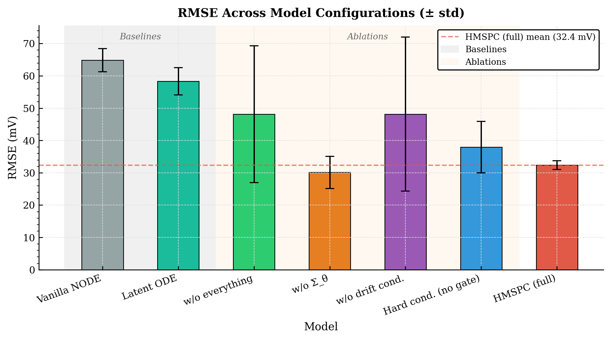
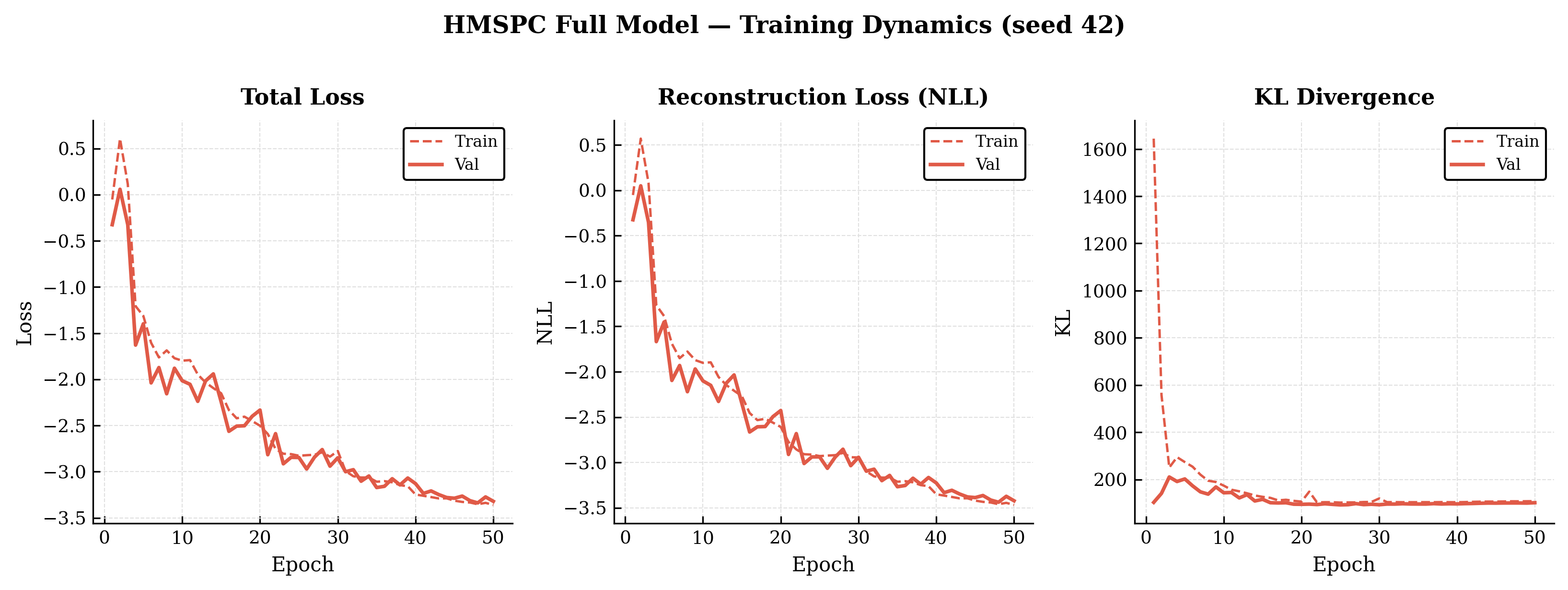
Figure 2 shows the training and validation curves for HMSPC (full) across total loss, reconstruction loss, and KL divergence for a single representative seed (seed 42).
6 Discussion
6.1 Drift Conditioning
The most noticeable finding from the ablation study is the variance of the ablation without drift conditioning. Removing drift conditioning (w/o drift cond.) produces a standard deviation of $\pm$ 23.84 mV, nearly 18$\times$ higher than HMSPC full ($\pm$ 1.34 mV), visible in the wide error bars of Figure 1. This suggests that input conditioning is not just improving accuracy on average, but actively stabilizing the latent trajectory during training. Without current and temperature to anchor the drift, the model must explain all regime-dependent structure through the latent state alone, making it sensitive to initialization and more prone to divergence across seeds.
6.2 Learned Gate
Hard conditioning without the learned gate (hard cond., no gate) achieves 37.97 mV RMSE compared to 32.37 mV for the full gated model, providing a meaningful gap despite using nearly identical architecture. The gate learns to modulate how strongly the inputs influence the drift at each step, effectively acting as a soft switch between input-driven and autonomous dynamics. This is particularly useful for battery data where inputs are highly informative during fast charge/discharge transitions but contribute less during rest periods.
6.3 Heteroscedastic Noise
Removing $\Sigma_\theta$ (w/o $\Sigma_\theta$) yields a slightly lower mean RMSE (30.11 vs 32.37 mV), but ECE degrades substantially from 0.078 to 0.159. The difference in RMSE is within one standard deviation and likely not statistically significant, while the calibration gap is large and consistent. For battery management systems, where overconfident predictions of voltage bounds can lead to unsafe operation, calibrated uncertainty is arguably more valuable than marginal RMSE gains. The heteroscedastic model also adds an auxiliary loss \(\mathcal{L}_{\text{unc}}\) that pushes $\sigma^2_{\text{obs}}$ to track residuals, providing an additional training signal beyond reconstruction alone.
6.4 Computational Cost
HMSPC incurs a 1.32$\times$ FLOPs overhead relative to Latent ODE (see Appendix A.4), driven primarily by the additional gate and delta networks in the drift. Given the 45% reduction in RMSE, this represents a favorable tradeoff, particularly since the additional parameters are small feed-forward networks rather than expensive attention or recurrent layers.
6.5 Latent Space Structure
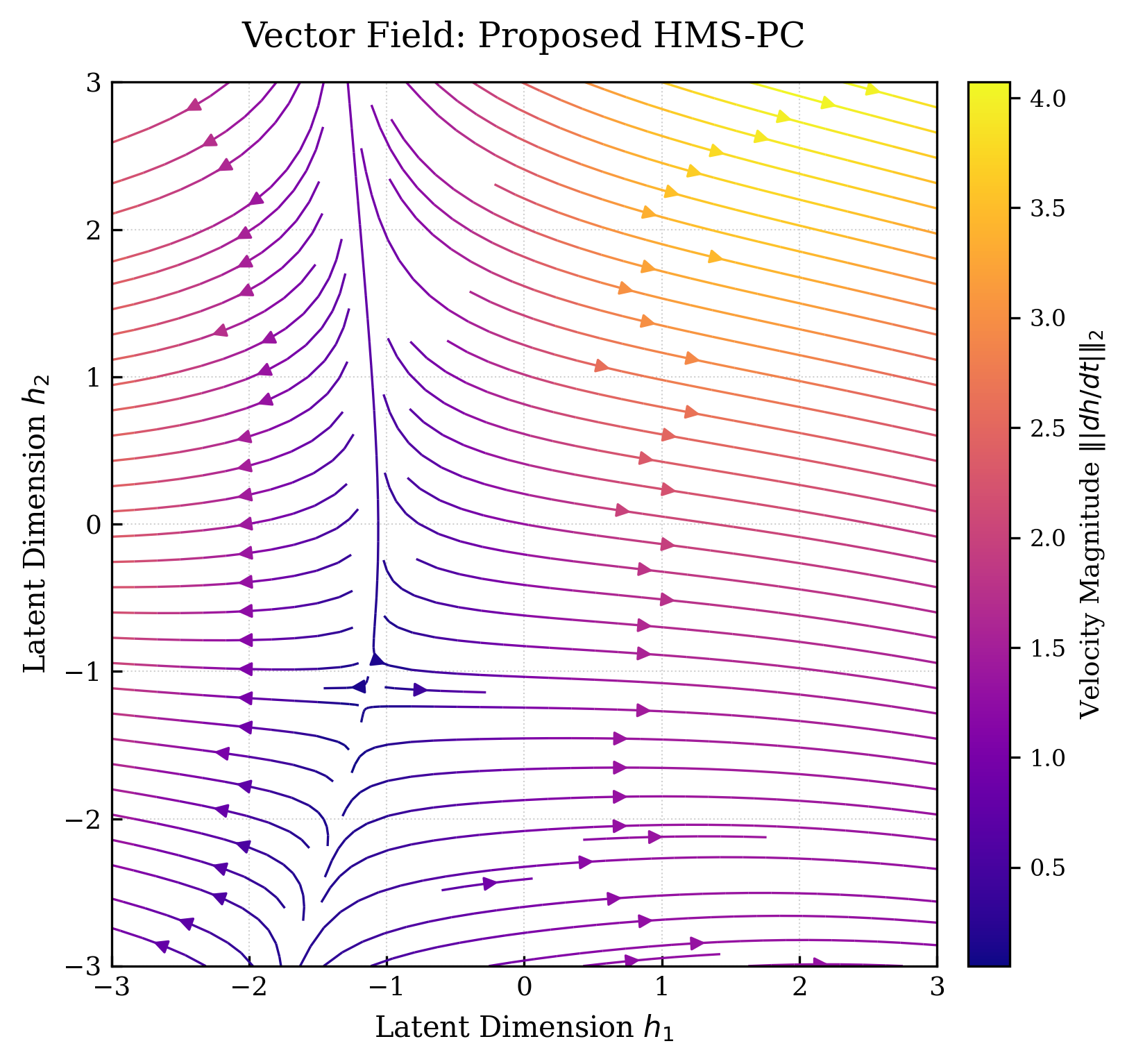
As a qualitative aside, Figure A1 in the Appendix visualizes the learned base drift $f_{\theta_1}$ projected onto the first two latent dimensions. The vector field reveals a structured attractor near $(-1, -1)$ in latent space, suggesting the model has learned a meaningful resting state that trajectories converge toward in the absence of input forcing. Whether this structure corresponds to interpretable battery states such as open-circuit equilibrium is an open question, and probing the geometry of the learned latent space represents an interesting direction for future work.
7 Conclusion
I presented HMSPC, a continuous-time latent variable model that extends the Latent ODE framework with three targeted improvements for battery voltage modeling. First, input-conditioned drift explicitly incorporates exogenous inputs current and temperature into the latent ODE, replacing purely autonomous dynamics with physically grounded evolution that reflects battery behavior (regime-dependent and driven by external operating conditions), providing a stronger inductive bias that contributed to empirical superiority over baselines. Second, a learned gating mechanism controls how strongly inputs influence the drift at each integration step, allowing the model to selectively incorporate input information rather than applying fixed conditioning throughout. Third, a heteroscedastic observation model replaces the fixed isotropic noise assumption of standard Latent ODEs with input and state-conditioned predictive variance, producing uncertainty estimates that adapt to the operating regime and remain calibrated across charging conditions.
Together these changes address the core mismatch between the Latent ODE’s inductive biases and the structure of battery data. Evaluated against Latent ODE and Vanilla Neural ODE baselines on the MIT-Stanford battery dataset across 5 seeds, HMSPC achieves a 45% reduction in RMSE alongside well-calibrated uncertainty estimates (ECE 0.078). Ablation studies confirm that each component contributes independently as removing drift conditioning destabilizes training, removing the gate degrades accuracy, and removing heteroscedastic noise collapses calibration. Future work should explore adaptive ODE solvers, multi-dataset evaluation across battery chemistries, and extensions toward direct state-of-health prediction from the learned latent trajectory.
All the code for this project has been open-sourced and can be accessed at HSMPC Github. Results are reproducible via fixed seeds, although all experiments were run on CPU (MacBook Pro) and the code has not been tested on GPU or other accelerator hardware. Minor numerical differences may occur across platforms.
Limitations
Single dataset
All experiments are conducted on the MIT-Stanford battery dataset. While this dataset is widely used and contains a diverse range of cycle lives and charging protocols, generalization to other battery chemistries, form factors, or cycling conditions remains unvalidated.
Forward Euler integration
HMSPC uses fixed-step forward Euler to discretize the latent ODE, which is crude relative to adaptive solvers such as dopri5 used in the original Neural ODE framework. All baselines use the same integrator, so comparisons are fair, but absolute performance may improve with higher-order methods.
Window-based evaluation
Models are trained and evaluated on fixed-length windows of 120 timesteps rather than full charge/discharge cycles. This simplifies batching but means the model has no explicit notion of cycle number or long-range degradation trends.
Small seed count
Results are averaged over 5 seeds. While this is standard for ablation studies, some ablation variants show high variance across seeds (notably w/o drift cond., $\pm 23.84$ mV), suggesting conclusions about those configurations should be interpreted cautiously.
No physics-based baseline
HMSPC is compared only against data-driven baselines. Hybrid physics-informed models such as equivalent circuit models augmented with neural corrections represent a natural comparison that is left to future work.
Ethics / deployment risks
Battery management systems are safety-critical as miscalibrated voltage predictions can contribute to thermal runaway, cell damage, or unsafe charging decisions. While HMSPC produces calibrated uncertainty estimates that make overconfidence less likely, no model should be deployed in a real BMS without extensive validation on the target hardware, chemistry, and operating conditions. Results here are on a research dataset under controlled conditions and should not be interpreted as production-ready. More broadly, improved battery models could accelerate electric vehicle adoption and grid storage deployment, which are net positives for decarbonization. The dataset used (MIT-Stanford) is publicly available and contains no personally identifiable information.
Appendix
A.1 Stopping gradients through \(\mu_{\text{obs}}\)
From the code:
residuals = (V - V_mean.detach()) ** 2
l_uncertainty = ((V_var - residuals).pow(2) * mask).sum() / mask.sum()
V_mean.detach() stops gradients through \(\mu_{\text{obs}}\) in $\mathcal{L}_{\text{unc}}$.
The reason is to keep the two objectives from interfering. \(\mathcal{L}_{\text{unc}}\) pushes \(\sigma^2_{\text{obs}}\) to match the squared residuals $(V - \mu_{\text{obs}})^2$. If you allowed gradients through $\mu_{\text{obs}}$, the uncertainty loss could inadvertently alter the mean prediction, since minimizing \((\sigma^2_{\text{obs}} - (V - \mu_{\text{obs}})^2)^2\) could partially be satisfied by making the residuals larger to match a poorly calibrated \(\sigma^2_{\text{obs}}\), rather than making \(\sigma^2_{\text{obs}}\) track the true residuals.
So the responsibilities are cleanly separated:
- \(\mathcal{L}_{\text{recon}}\) trains $\mu_{\text{obs}}$ to predict well
- \(\mathcal{L}_{\text{unc}}\) trains $\sigma^2_{\text{obs}}$ to match the residuals from that mean
A.2 Hyperparameters
All hyperparameters shared across every model (NODE, Latent ODE, HMSPC and all ablations):
| Hyperparameter | Value |
|---|---|
| Optimizer | Adam |
| Learning rate | $10^{-3}$ |
| LR scheduler | ReduceLROnPlateau (factor $0.5$, patience $3$) |
| Gradient clipping | max norm $1.0$ |
| Max epochs | $50$ |
| Early stopping patience | $10$ |
| Batch size | $16$ |
| Latent dim $d_z$ | $32$ |
| Hidden dim $d_H$ | $64$ |
| Window size | $120$ |
| Windows per cell | $50$ |
| Quantile bins (stratified split) | $20$ |
| Train/val/test split | $70/15/15$ |
| Linear init | Xavier uniform |
| GRU init | Orthogonal |
| Bias init | Zero |
HMSPC and Latent ODE additionally use KL annealing (Vanilla NODE has no variational objective):
| Hyperparameter | HMSPC | Latent ODE |
|---|---|---|
| KL warmup epochs | $15$ | $10$ |
| $\beta_{\text{KL}}$ target | $10^{-3}$ | $10^{-3}$ |
HMSPC only:
| Hyperparameter | Value |
|---|---|
| $\beta$ target | $0.3$ |
| $\beta$ warmup epochs | $15$ |
A.3 Stratified Data Split
Cells are stratified by cycle life to ensure all splits contain a representative range of battery lifetimes. Cells with missing cycle life labels are assigned to training only.
valid_cells = []
nan_cells = []

for cid in cell_ids:
    cycle_life = float(data_dict[cid]["cycle_life"])
    if np.isnan(cycle_life):
        nan_cells.append(cid)
    else:
        valid_cells.append((cid, cycle_life))

# sort by cycle life and split into 20 quantile bins
valid_cells.sort(key=lambda x: x[1])
bins = np.array_split(valid_cells, n_bins)  # n_bins = 20

for bin_cells in bins:
    bin_cells = list(bin_cells)
    rng.shuffle(bin_cells)

    n_bin = len(bin_cells)
    n_train = int(round(0.70 * n_bin))
    n_val = int(round(0.15 * n_bin))

    train_cells.extend(cid for cid, _ in bin_cells[:n_train])
    val_cells.extend(cid for cid, _ in bin_cells[n_train : n_train + n_val])
    test_cells.extend(cid for cid, _ in bin_cells[n_train + n_val :])

# NaN-life cells go to train only
train_cells.extend(nan_cells)
A.4 Computational Cost
| Model | Params $\downarrow$ | FLOPs $\downarrow$ | Relative FLOPs |
|---|---|---|---|
| HMSPC (full) | $57.80\text{K}$ | $6.39\text{M}$ | $1.32\times$ |
| w/o $\Sigma_\theta$ | $57.80\text{K}$ | $6.39\text{M}$ | $1.32\times$ |
| hard cond. (no gate) | $55.49\text{K}$ | $6.12\text{M}$ | $1.26\times$ |
| w/o drift cond. | $47.01\text{K}$ | $5.12\text{M}$ | $1.06\times$ |
| Latent ODE | $44.70\text{K}$ | $4.85\text{M}$ | $1.00\times$ |
| Vanilla Neural ODE | $14.95\text{K}$ | $1.74\text{M}$ | $0.36\times$ |
A.5 HMSPC Vector Field
References
[1] Rubanova, Y., Chen, R. T. Q., & Duvenaud, D. (2019). Latent ODEs for Irregularly-Sampled Time Series. NeurIPS.
[2] K. A. Severson, P. M. Attia, N. Jin, N. Perkins, B. Jiang, Z. Yang, M. H. Chen, M. Aykol, P. K. Herring, D. Fraggedakis, M. Z. Bazant, S. J. Harris, W. C. Chueh, and R. D. Braatz. “Data-driven prediction of battery cycle life before capacity degradation.” Nature Energy, 4:383–391, 2019.
[3] Chen, R. T. Q., Rubanova, Y., Bettencourt, J., & Duvenaud, D. (2018). Neural Ordinary Differential Equations. NeurIPS.
[4] Cho, K., van Merrienboer, B., Gulcehre, C., Bahdanau, D., Bougares, F., Schwenk, H., & Bengio, Y. (2014). Learning Phrase Representations using RNN Encoder-Decoder for Statistical Machine Translation. EMNLP.
[5] Glorot, X., & Bengio, Y. (2010). Understanding the difficulty of training deep feedforward neural networks. AISTATS.
[6] Saxe, A., McClelland, J., & Ganguli, S. (2014). Exact solutions to the nonlinear dynamics of learning in deep linear neural networks. ICLR.
[7] Kingma, D. P., & Welling, M. (2013). Auto-Encoding Variational Bayes. ICLR.
[8] Kingma, D. P., & Ba, J. (2014). Adam: A Method for Stochastic Optimization. ICLR.
[9] Guo, C., Pleiss, G., Sun, Y., & Weinberger, K. Q. (2017). On Calibration of Modern Neural Networks. ICML.