Beyond Black Boxes: A Framework for Building Rigorous AI for Volatility Forecasting
Code available at Garch-LSTM Volatility Github
The Problem with Naive Neural Nets for Financial Modelling
In quantitative finance, many hail neural networks as a mystical system that, given enough training, can predict anything. Although neural networks are impressive, they are often opaque and confidently wrong. It’s easy to train an LSTM or even a Transformer on price data and claim 95% accuracy. However, it’s harder to answer the question: is the model gathering signal, or is it memorizing noise?
I recently built a volatility forecasting system that made me confront this question head-on. The results might change how you think about using Artificial Intelligence in financial modelling.
The Hybrid Approach: GARCH Meets LSTM
Traditional finance has long used GARCH models, statistical workhorses that capture local volatility clustering effectively but struggle with complex, non-linear patterns. Modern AI has LSTMs, excellent at learning temporal dependencies but often lacking statistical rigor and prone to overfitting past data.
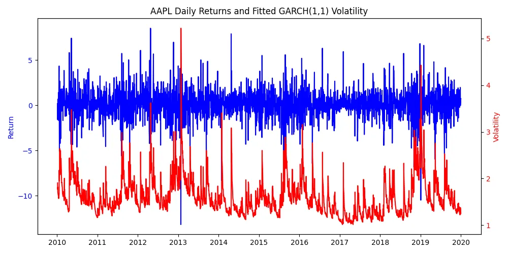
What if we combined them?
The system integrates:
- GARCH models for conditional volatility
- LSTM networks for temporal pattern recognition
- Multiple technical indicators (RSI, MACD, moving averages)
- Statistical features (rolling skewness, kurtosis, Hurst exponent)
The validation was however the most insightful part of this project.
Monte Carlo Permutation Testing
After training models on 30 years of data across 8 stocks, I faced the critical question: are these models actually predictive, or could they perform just as well on random data? I implemented ideas from Evidence-Based Technical Analysis by David Aronson, notably for testing if the model generalized to out-of-sample volatility predictions.
Namely, I used Aronson’s Monte Carlo Permutation Test. This statistical method creates synthetic datasets by:
- Permuting returns (destroying temporal structure but preserving distribution)
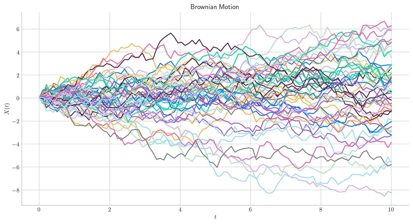
- Generating Brownian motion (complete randomness with similar statistics)
How It Works in the Code
The code generates two types of synthetic data:
- Permuted Returns: Like shuffling a deck of cards.
- Real data:
[0.01, -0.02, 0.015, -0.008, ...](actual sequence) - Synthetic:
[-0.008, 0.01, -0.02, 0.015, ...](random order) - Preserves the same numbers (same distribution) but destroys all temporal patterns and dependencies.
- Real data:
- Brownian Motion: Complete randomness.
- Generated from a normal distribution with the same mean and variance.
- No relationship to actual market behavior whatsoever.
The Comparison
For each stock, you compare the loss metric directly:
- Real Data MAE: 0.001155
- Synthetic Data MAE (average): 0.002487
The Statistical Test
I ran this comparison more than 100 times (preferably >1000 times but due to limited compute I only did 100 for each) and counted:
- Number of times synthetic MAE $\le$ real MAE: 0 out of 100
Hence, the estimated p-value $\approx 0$ (no synthetic sample outperformed the real data in 100 trials).
What the Results Actually Mean
Case 1: Significant Result ($p \le 0.01$)
p-value $\approx 0$
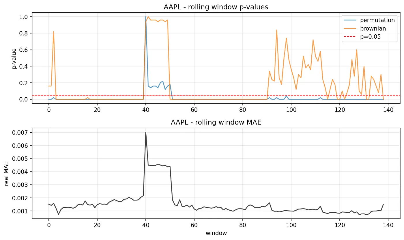
This p-value was calculated after I tested with AAPL stock. In 100 attempts with completely random data, the model never performed as well as it did on real AAPL data. This outcome is extremely unlikely to occur by chance, roughly equivalent to getting 100 heads in a row when flipping a fair coin ($\approx 7.9 \times 10^{-31}$ probability under pure noise). This strongly suggests that the model has learned genuine, reproducible patterns rather than random fluctuations.
Case 2: Marginally/Non-Significant Result ($p > 0.01$)
p-value = 1.0000
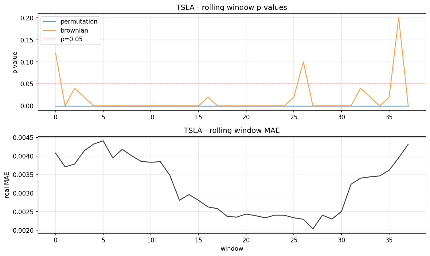
I obtained this value after testing with TSLA stock. The model performed just as well on random data as it did on real TSLA data. Hence, it’s probably not learning any real patterns specific to TSLA.
Why Your Metrics Might Be Lying to You
The uncomfortable truth in quantitative finance in particular is that good performance metrics alone don’t prove your model actually works.
Without proper statistical testing:
- MAE = 0.001155 suggests the model can accurately predict volatility, yet it may fall apart in out-of-sample use due to inadequate statistical testing.
With Monte Carlo Permutation Testing:
- You can confidently state that the model achieves MAE = 0.001155, and statistical testing confirms this performance is genuine ($p < 0.0001$), not just random luck.
The reason we need this rigorous testing is that financial data naturally contains patterns that can fool naive models. Even a simple model can appear successful because it’s accidentally capturing:
- Autocorrelation: Where today’s returns influence tomorrow’s.
- Volatility clustering: The tendency for big moves to cluster together.
- Mean reversion: Prices eventually returning to their historical averages.
These aren’t sophisticated patterns your model learned: they’re basic statistical properties of markets that even random models can stumble upon even though they are not statistically proven to always occur.
What the Data Revealed
After running the test script:
- 6 out of 8 stocks showed statistically significant predictive power: but two didn’t.
- The volatility of TSLA and BA proved to be too hard to model, most likely due to the stock prices being largely determined due to news rather than past patterns. I’ve attached the rolling window p-value and MAE for both AAPL (which the LSTM generalized to well), as well as the TSLA (which gave poor results).
The Feature Importance Surprise
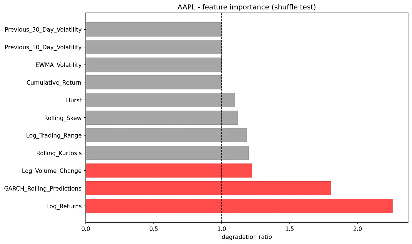
When I tested which features mattered most by shuffling them, the results were mostly consistent across stocks:
- The GARCH predictions (the traditional finance component) proved to be the second most important feature in almost every stock.
- This wasn’t just AI outperforming traditional methods; it was AI learning to leverage traditional methods.
- I also saw that some features were redundant, which I am planning to remove in future training.
Stress Testing Reality
Financial models need to work when markets break from normal patterns. The stress tests using heavy-tailed t-distributions revealed how the models would perform during extreme volatility.
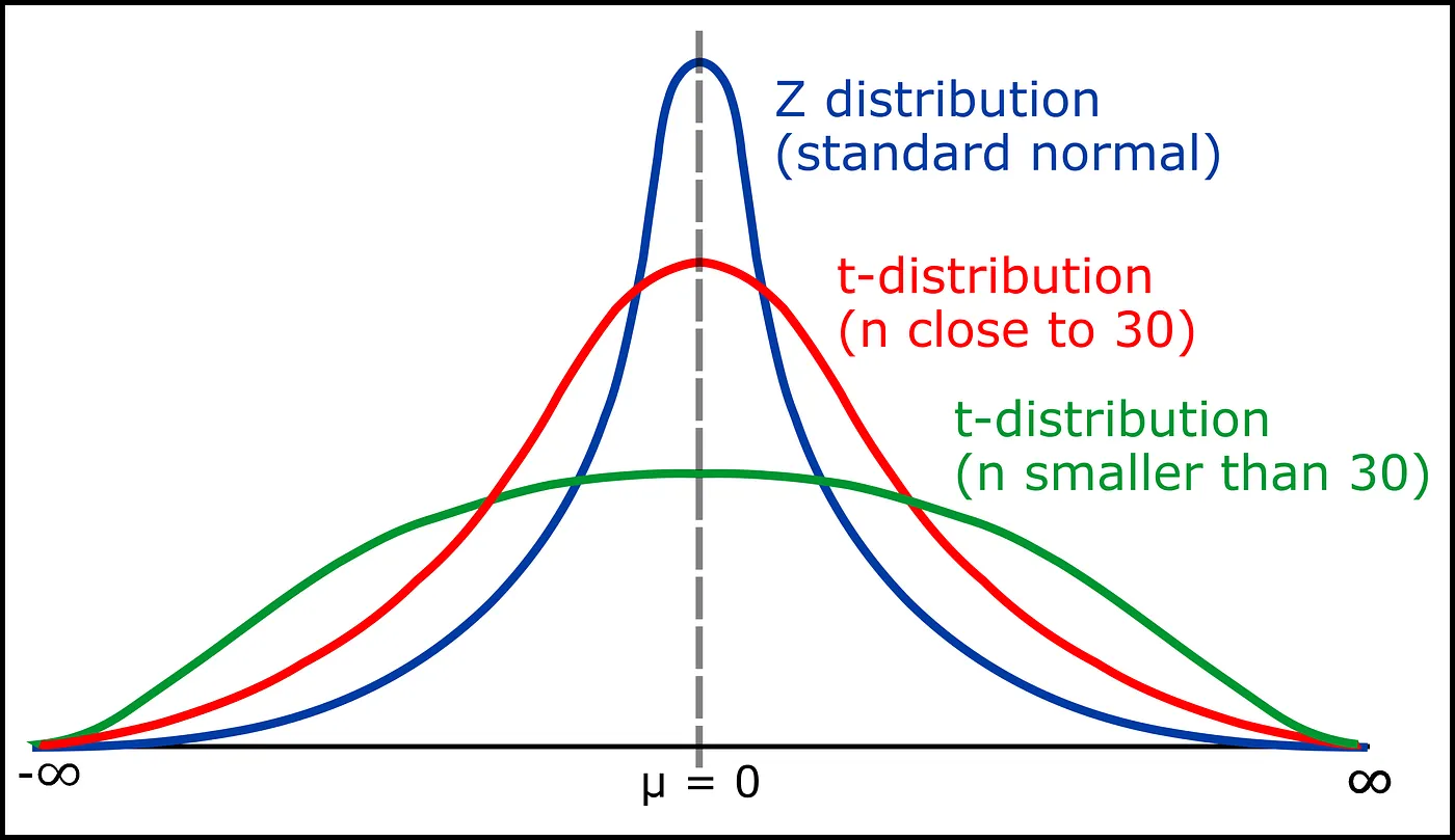
Stress test results:
- AAPL: 0.002547 (120% higher error)
- JPM: 0.002377 (145% higher error)
The models remained functional under stress, but with predictably degraded performance which is what is expected from a robust system.
The Training Journey
Watching the models train was also very insightful. I started off with just S&P 500 close prices, but eventually switched to a multi-stock training setup. I also added early stopping to prevent overfitting where the model begins to learn the noise of the training set rather than useful signal.
The training logs showed the gradual improvement and the importance of early stopping:
Epoch 54 | Train: -0.3835 | Test: -0.5057 (1)
Epoch 55 | Train: -0.3885 | Test: -0.4954 (2)
...
Epoch 116 | Train: -0.5335 | Test: -0.6070 (20)
Early stopping at epoch 116
The best models weren’t the ones that trained the longest, but the ones that stopped at the right moment, typically around 100–120 epochs.
model = ProbLSTM(
    input_size=X_train.shape[2],
    hidden_size=64,
    num_layers=2,
    dropout=0.5,
    num_gaussians=1,
).to(device)
I also added a high level of regularization such as the 0.5 dropout and 1e-5 for weight decay. Through extensive testing, these values gave the best results (for final MAE in training) as well as for passing the testing script by minimizing overfitting.
What This Means for AI in Finance
This project taught me several crucial lessons:
- Statistical rigor isn’t optional: Without proper testing, you’re just using wishful thinking with fancy algorithms.
- Hybrid approaches work: Traditional finance models and AI can complement each other beautifully.
- Not all stocks are predictable: Some securities like TSLA might be inherently less forecastable.
- Feature engineering matters: The GARCH component proved critical despite the neural network’s complexity, and to a lesser extent Kurtosis, skew, and Hurst.
The Code That Made It Possible
The entire system is built with Python, using:
- PyTorch for the LSTM implementation
- ARCH for GARCH modeling
- yfinance for data acquisition
- Custom statistical testing frameworks
Moving Forward
I am looking to:
- Test on more asset classes (currencies, commodities)
- Incorporate macroeconomic data
- Build ensemble approaches
- Explore alternative architectures like Transformers or attention heads
However, the foundation is solid. The AI system doesn’t just make predictions, but can statistically defend why those predictions might be meaningful.
Conclusion
Building a model for quantitative finance isn’t just an act of prediction but an act of restraint. It is often easy to assume the market is deterministic, when in reality it is stochastic.
All the code, tests, and results are open-sourced so you can reproduce every step. I’ve uploaded my code for this journey through quantitative finance on GitHub here: garch-lstm-volatility. Do check it out if you are interested.